Is the Expected Value of a Continuous Random Variable the Mean
Expected Value of Continuous Random Variables
Theory
Definition 37.1 (Expected Value of a Continuous Random Variable) Let \(X\) be a continuous random variable with p.d.f. \(f(x)\). Then, the expected value of \(X\) is defined as \[\begin{equation} E[X] = \int_{-\infty}^\infty x \cdot f(x)\,dx. \tag{37.1} \end{equation}\]
Compare this definition with the definition of expected value for a discrete random variable (22.1). We simply replaced the p.m.f. by the p.d.f. and the sum by an integral.
Example 37.1 (Expected Value of the Uniform Distribution) Let \(X\) be a \(\text{Uniform}(a, b)\) random variable. What is \(E[X]\)?
First, the p.d.f. is \[ f(x) = \begin{cases} \frac{1}{b-a} & a \leq x \leq b \\ 0 & \text{otherwise} \end{cases}, \] which is non-zero only between \(a\) and \(b\). So, even though (37.1) says we should integrate from \(-\infty\) to \(\infty\), the integrand will only be non-zero between \(a\) and \(b\).
\[\begin{align*} E[X] &= \int_a^b x \cdot \frac{1}{b-a} \,dx \\ &= \frac{1}{b-a} \left. \frac{x^2}{2} \right]_a^b \\ &= \frac{1}{b-a} (b^2 - a^2) \frac{1}{2} \\ &= \frac{a + b}{2}. \end{align*}\]
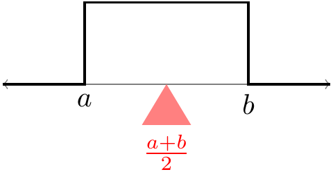
This is just the midpoint of the possible values of this uniform random variable. This is clearly the point where the p.d.f. would balance, if we put it on a scale.

Figure 37.1: Expected Value of the Uniform Distribution
Example 37.2 (Expected Value and Median of the Exponential Distribution) Let \(X\) be an \(\text{Exponential}(\lambda)\) random variable. What is \(E[X]\)? Does the random variable have an equal chance of being above as below the expected value?
First, we calculate the expected value using (37.1) and the p.d.f. of the exponential distribution (35.1). This is an exercise in integration by parts. \[\begin{align*} E[X] &= \int_0^\infty x \cdot \lambda e^{-\lambda x} \,dx \\ &= -x e^{-\lambda x} \Big|_0^\infty - \int_0^\infty -e^{-\lambda x}\,dx \\ &= \ (-0 + 0) - \underbrace{\frac{1}{\lambda} e^{-\lambda x} \Big|_0^\infty}_{0 - \frac{1}{\lambda}} \\ &= \frac{1}{\lambda} \end{align*}\]
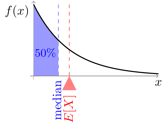
Now, let's calculate the probability that the random variable is below expected value. \[ P(X < E[X]) = P(X < \frac{1}{\lambda}) = \int_0^{1/\lambda} \lambda e^{-\lambda x}\,dx = 1 - e^{-1} \approx .632. \] The random variable does not have an 50/50 chance of being above or below its expected value.
The value that a random variable has an equal chance of being above or below is called its median. To calculate the median, we have to solve for \(m\) such that \[ P(X < m) = 0.5. \] (Equivalently, we could solve \(P(X > m) = 0.5\). It also doesn't matter whether we use \(<\) or \(\leq\), since this is a continuous random variable, so \(P(X = m) = 0\).)
Calculating the probability in terms of \(m\), we have \[ 0.5 = P(X < m) = \int_0^m \lambda e^{-\lambda x}\,dx = 1 - e^{-\lambda m}. \] Solving for \(m\), we see that the median is \(-\log(0.5) / \lambda\). (Note: \(\log\) here is the natural logarithm, base \(e\).)

Figure 37.2: Mean vs. Median of the Exponential Distribution
Formulas for the variance of named continuous distributions can be found in Appendix A.2.
Essential Practice
-
The distance (in hundreds of miles) driven by a trucker in one day is a continuous random variable \(X\) whose cumulative distribution function (c.d.f.) is given by: \[ F(x) = \begin{cases} 0 & x < 0 \\ x^3 / 216 & 0 \leq x \leq 6 \\ 1 & x > 6 \end{cases}. \]
- Calculate \(E[X]\), the expected value of \(X\).
- Calculate the median of \(X\).
- Sketch a graph of the p.d.f., along with the locations of the expected value and median.
-
Suppose that an electronic device has a lifetime \(T\) (in hours) that follows an \(\text{Exponential}(\lambda=\frac{1}{1000})\) distribution.
- What is \(E[T]\)?
- Suppose that the cost of manufacturing one such item is $2. The manufacturer sells the item for $5, but guarantees a total refund if the lifetime ends up being less than 900 hours. What is the manufacturer's expected profit per item?
Source: https://dlsun.github.io/probability/ev-continuous.html
0 Response to "Is the Expected Value of a Continuous Random Variable the Mean"
Post a Comment